What happens inside a neural network? How are values assigned to a neuron? Let’s try to walk through each step of a neural network pipeline.

Adding basics about a neural network will make this post lengthier than it already is. So, this is not a basic - what is a neural network guide. Please, go through following articles about what a neural network is and it’s two main entities:

• Perceptron
• Gradient Descent

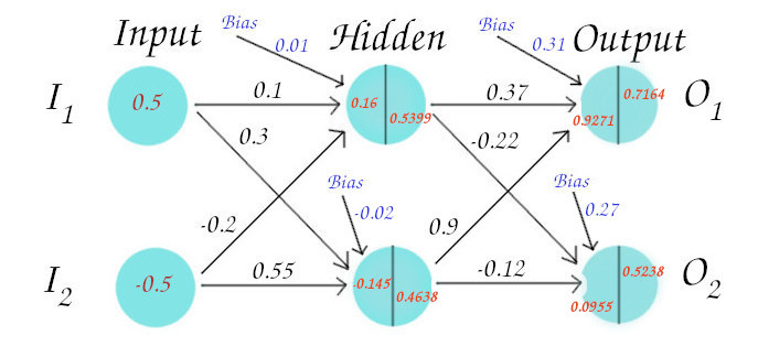
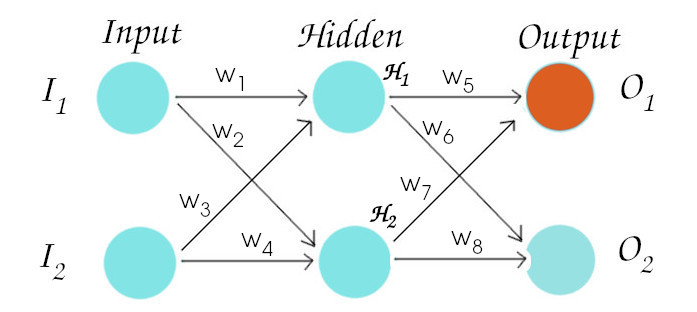
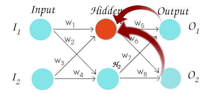
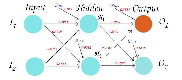
What we will do today is, consider the following neural network as an example and run through every step from start to end, of how the network learns while training.

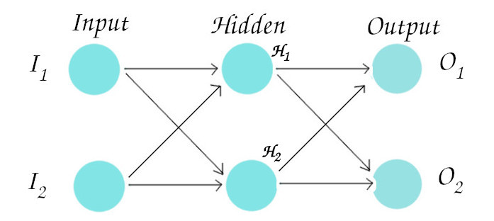
This particular network consists of 3 layers i.e input, hidden and output layer and 2 neurons in each layer. We take only two neurons in each layer in our example because if we understand the sole concept, adding neurons and layers is a child’s play.

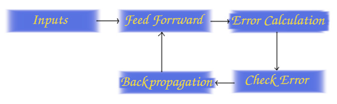
Let’s start with a simple pipeline, the way a Neural Network learns:

Inputs:

Usually, inputs are the feature vectors of some kind. If you are performing a image classification as a cat or dog classifier, the input is the collection of values which represent features of some kind of the image that is in your training data. The simplest feature vector extractor is local binary pattern in which the vector is the collection of 0’s and 1’s and the size of the vector is equal to (A multiplied by B), if the resolution of image is AxB. You can go through more advanced feature extraction techniques if you like, but we will not cover that here.

Feed Forward:

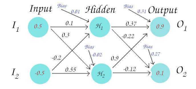
Lets’ consider the following neural network with input vector (0.5, -0.5), which means the first neuron of the input layer will have value 0.5 and second neuron will have -0.5. Each neuron has a bias value associated with it so that it can help, fire up the neurons if weights and inputs are not sufficient. Now, to have some weights to work with we randomly initialize the weights here for the sake of simplicity but in real world, there are things we should consider during weight initialization. You can go through weight initialization techniques in a neural network to know about why we should not use same weights for all neurons or simply random values as weights.

Let’s take a concept of perceptron analysis and move forward. Remember as we discussed in perceptron section, each neuron has two values in it, the Net Summed (Z) and the activated (S) value.
For the 1st neuron of 2nd (hidden) layer, we calculate the Net Summed value and activated value as follows:

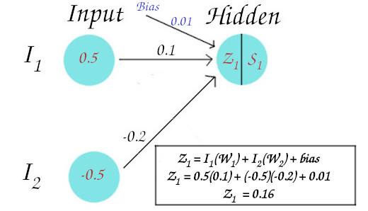
As we know the Net value (Z₁) is calculated by using following:

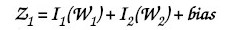
We obtain Z₁ = 0.16, as shown in the above figure.
Now we need some activation function helps to make the output non-linear. The function to calculate the Net Value (Z) is just the equation of straight line (y=mx+c) which is a linear function. And what activation function does is, give nonlinearity to it. Know more detail about this in perceptron topic. Here, we use a sigmoid activation function for demonstration purpose.

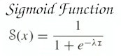where λ=Scaling factor and I=Net value (Z) of that neuron, which we calculated earlier.

The calculation of the activated value of 1st neuron of hidden layer is shown in the figure below:

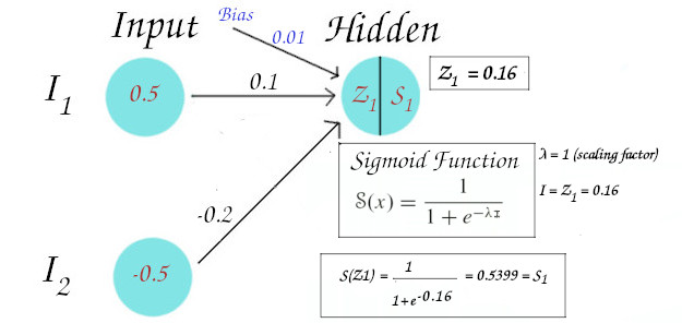
So we get the Net value (Z₁) = 0.16 and activated value (S₁) = 0.5399.

Now, this activated value becomes imput for the next neuron. In this way, we move forward until we finish calculating for the neurons of the output layer. In the figure below all the red colored values are the calculated values for all Z and S.

Error Calculation:

How much does the output of the final layer neurons in one pass, vary from our expected output? There are many methods to calculate errors but here we use a mean squared error calculation. We will use this while doing the backpropagation.

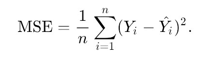where Y is the expected output, Y^{^} is the actual or calculated output and n is the number of training samples.

Backpropagation (Output to Hidden):

Now that we have propagated forward, it is time to propagate backwards, using the gradient decent algorithm we mentioned before. This is where the network learns. What we do basically is, we calculate the error value for the neurons in output layer and according to how much the error is, we tweak the weights, propagate forward again and so on until we get minimum error.

Let’s start. So, till now we know that we have to change the weight according to the error. So we have differentiated error with respect to weight. But we can not do it directly and here is why:

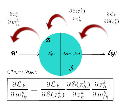
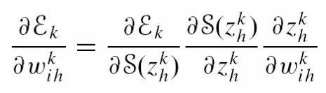
The δ(y) value is not directly related to the weight value as we can see in the figure above. The weight is related directly to Z, Z to S and S to δ(y). So what we have to do is we have to apply a simple chain rule to differentiate (error) w.r.t (weight). First, we have to differentiate error w.r.t (S), (S) w.r.t (Z) and (Z) w.r.t (W) and multiply them as follows:

So, let’s start updating weight (w₅) for the 1st neuron of the output layer.

Assigning the previously calculated values in forward propagation, we have:

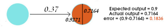
NOTE: The error calculated here is just a simple error, we will calculate mean squared error later.

Let’s take it step by step and operate 3 parts of the formula separately. Following are the derivation of each term, individually:

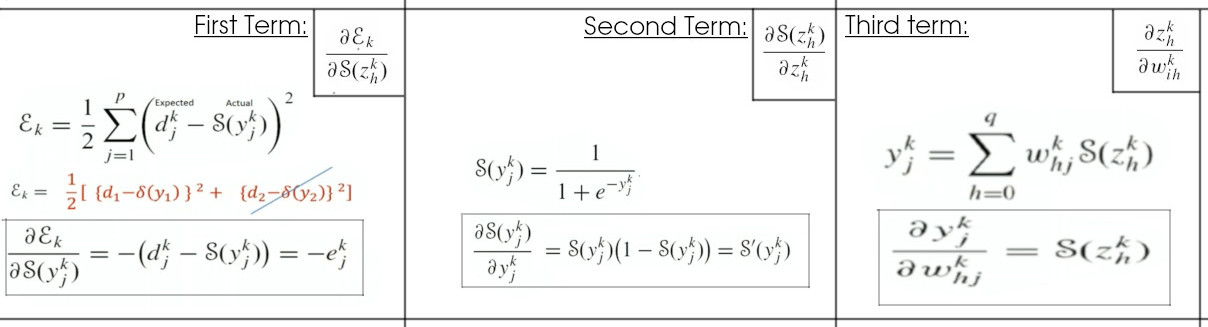
In simple terms, the values of those terms derives to these values:

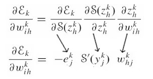
Now, let’s put the respective terms from the values we calculated when feed forwarding. It goes like this:

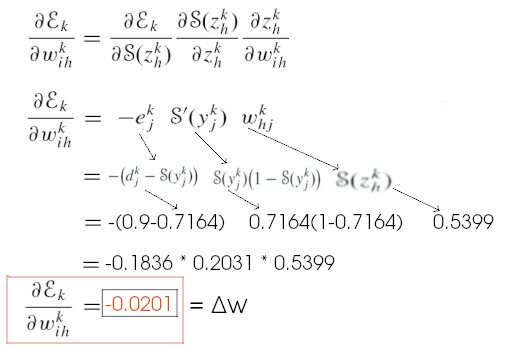
Now, we have the value for ΔW, we can update the weight by the weight update rule like this:

This is where learning rate is used. For our particular example, we take learning rate η=1.2 but in real world this value cannot be so high because then, the network will never learn. More details can be found in the Gradient Descent section.

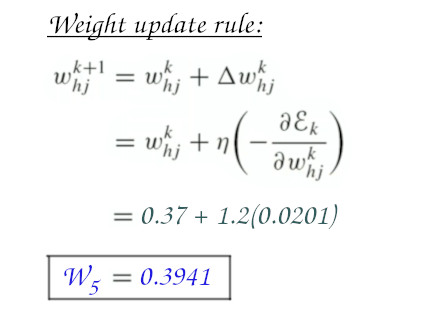
So, we have the previous weight W₅ = 0.37 and ΔW = -0.0201. The new weight value for W₅, as calculated in above figure, will be 0.3941.

Backpropagation (Hidden to Input):

To update the weights of other neurons except the output neurons is a little bit different. This is because each of the output neurons only have effect on one error value but if we take 1st neuron of the hidden layer, it effects both neurons of the output layer. So we backpropagate through both of the outputs. Previously, we followed this path:

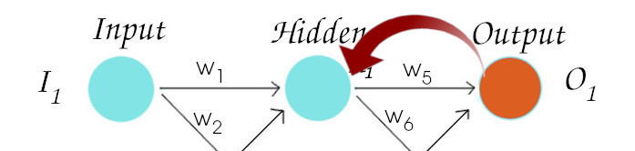
Now, we backpropagate through following path to update weight W₁ so a little bit of extra steps to follow.

Following formula is used to find out the ΔW for W₁. Here, p is the number of path we come through when bacjpropagating to that particular neuron. Simply put, it is the number of neurons in our output layer. So we have p=2.

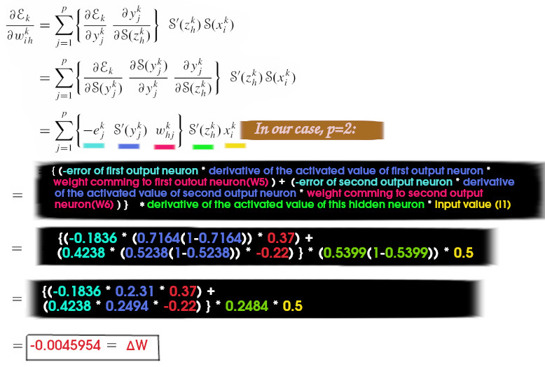
So, in this way we have found the ΔW₁ = -0.0045954 and now it is time to obtain the new weight for W₁ using the weight update rule as we did previously.

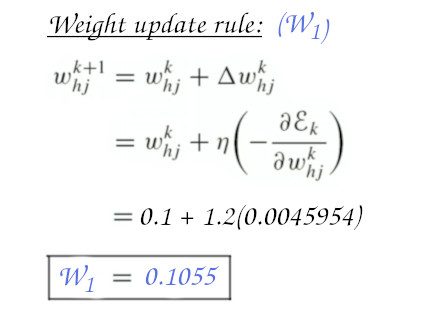
In this way, we calculate the new weight values for each weigh associated with all neurons in hidden and output layer and the final calculated result will be as shown below:

We now have finished backpropagating. Now, we repeat all this feed forward and backpropagation until we reach a decently lesser error value as shown in this previous pipeline.

We have finished a basic walkthrough of a neural network and backpropagation algorithm. A network can learn from this but there are many more optimization techinques which are used widely throughout the globe to minimize the error and yield a highly accurate model. This is it for now and we can discuss about those optimization alogithm later in another post.

Here is my implementation of an Artificial Neural Network in C++ using this concept.